HLookup Functions

=HLOOKUP(Value you want to look up, range where you want to lookup the value, the row number in the range containing the return value, Exact Match or Approximate Match – indicated as 0/FALSE or 1/TRUE).

• value The value to search for in the first row of the table.
• table Two or more rows of data that is sorted in ascending order.
• index_number The row number in table from which the matching value must be returned. The first row is 1.
• approximate_match [optional] Enter FALSE to find an exact match. Enter TRUE to find an approximate match. If this parameter is omitted, TRUE is the default.

• If you specify FALSE for the approximate_match parameter and no exact match is found, then the HLOOKUP function will return #N/A.
• If you specify TRUE for the approximate_match parameter and no exact match is found, then the next smaller value is returned.
• If index_number is less than 1, the HLOOKUP function will return #VALUE!.
• If index_number is greater than the number of row in table, the HLOOKUP function will return #REF!.

VLOOKUP is designed to retrieve data in a table organized into vertical rows, where each row represents a new record. The "V" in VLOOKUP stands for vertical:

When you use VLOOKUP, imagine that every column in the table is numbered, starting from the left. To get a value from a particular column, simply supply the appropriate number as the "column index":

VLOOKUP has two modes of matching: exact and approximate, which are controlled by the 4th argument, called "range_lookup". Set range_lookup to FALSE to force exact matching, and TRUE for approximate matching.

Important: range_lookup defaults to TRUE, so VLOOKUP will use approximate matching by default:
=VLOOKUP(value, table, column) // default, approximate match
=VLOOKUP(value, table, column, TRUE) // approximate match
=VLOOKUP(value, table, column, FALSE) // exact match

In most cases, you'll probably want to use VLOOKUP in exact match mode. This makes sense when you have a unique key to use as a lookup value, for example, the movie title in this data:

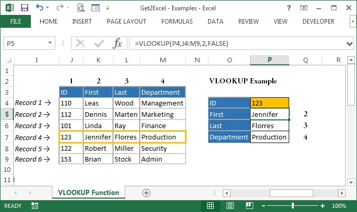
The formula in P5 to lookup first name based on an exact match of ID is:
=VLOOKUP(P4,J4:M9,2,FALSE) // FALSE = exact match

You'll want to use approximate mode in cases when you're looking for the best match, not an exact match. A classic example is finding the right commission rate based on a monthly sales number. In this case, you want VLOOKUP to get you the best match for a given lookup value. In the example below, the formula in D5 performs an approximate match to retrieve the correct commission.

The formula in P5 to lookup first name based on an approximate match of ID is:
=VLOOKUP(P4,J4:M9,2,TRUE) // TRUE = approximate match

Note: your data must be sorted in ascending order by lookup value when you use approximate match mode with VLOOKUP.